ETL pipeline, source snapshots, and computed signals

The pipeline

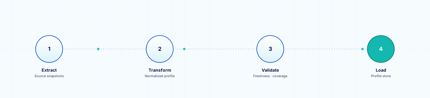
Four steps, in order, every run.

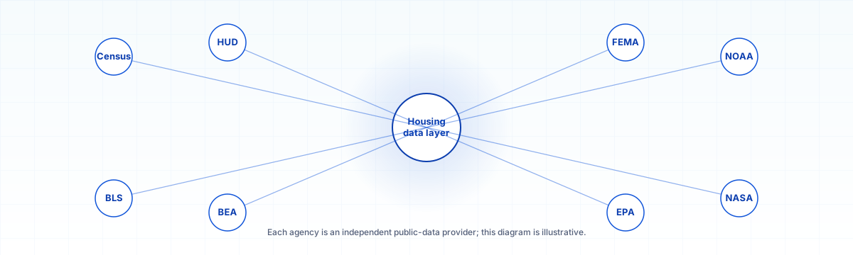
Eight independent federal data agencies feed this project's data layer. The diagram is illustrative; each agency publishes its own data on its own cadence under its own terms.

1. Step 1

   Extract

   Each registered source adapter loads a canonical SourceSnapshot for every supported geography. Snapshots carry an id, source id, dataset name, period, retrieved/release dates, source URL, update frequency, confidence, and the raw metric values themselves.

2. Step 2

   Transform

   The transform step assembles a NormalizedMarketProfile per geography: metrics keyed by stable ids (population, medianGrossRent, homePriceIndex, …), computed signal scores, an aggregated source attribution roster, freshness info, and a coverage report.

3. Step 3

   Validate

   Four validators run on the pipeline output: freshness (age vs. cadence), completeness (required metrics per report), geography (required identity fields), and metrics (units present, no impossible values). Findings are warnings — not build failures — and surface on /data-status.

4. Step 4

   Load

   Phase 3 'load' writes profiles into an in-memory store keyed by geography id. The interface is intentionally db-shaped so a Postgres / KV / S3 loader can replace it without changing the rest of the pipeline.

Why public data

Background from the U.S. Census Bureau on the American Community Survey — the survey program behind the ACS 5-year tables this project uses. Embedded as agency context, not as a partnership or endorsement.

Core concepts

Signal formulas

• Affordability signal

  computed signal

  rentBurden = annualGrossRent / medianHouseholdIncome; score = clamp(round((0.30 − rentBurden) / 0.30 × 100 + 50), 0, 100)

  rentBurden = 0.30 → 50. Lower burden → higher score.

  Inputs: ACS medianGrossRent, ACS medianHouseholdIncome

• Supply signal

  computed signal

  intensity = (trailing12PermitTotal / housingUnits) × 1,000; score = clamp(round(intensity / 0.6), 0, 100)

  ~60 permits per 1,000 existing units per year ≈ 100.

  Inputs: Census BPS trailing-12 permits, ACS housing units

• Price momentum signal

  computed signal

  score = clamp(round(50 + hpiYoYChangePct × 5), 0, 100)

  0% YoY → 50. +10% → 100. −10% → 0.

  Inputs: FHFA HPI YoY % change

• Climate risk signal

  computed signal

  score = round(femaNriRiskIndex) // 0-100, higher = more hazard exposure

  Surfaces FEMA's National Risk Index directly — no transformation. Direction follows FEMA: higher means more exposure. Kept separate from the positive signals so the semantics don't blur.

  Inputs: FEMA NRI naturalHazardRiskIndex (county-level)

• Job market signal

  computed signal

  level = clamp((8.5 − unemploymentRate) / (8.5 − 2.5) × 100, 0, 100); trend = clamp((1.0 − unemploymentRateChange12m) / 2.0 × 100, 0, 100) (missing → 50); jobMarket = round(level × 0.7 + trend × 0.3)

  Positive 0-100 signal. Lower unemployment and a falling 12-month trend both raise it. Level weighted 70%, trend 30%. ≤2.5% → 100 on level; ≥8.5% → 0. −1.0 ppt YoY → 100 on trend; +1.0 ppt → 0.

  Inputs: BLS LAUS unemploymentRate, unemploymentRateChange12m (county-level)

• Economic strength signal

  computed signal

  incomeGrowth = clamp((pcpiGrowthYoY + 2) / 8 × 100, 0, 100) [weight 0.45]; incomeLevel = clamp((perCapitaPersonalIncome − 40000) / 60000 × 100, 0, 100) [weight 0.35]; gdpGrowth = clamp((regionalGdpGrowthYoY + 2) / 8 × 100, 0, 100) [weight 0.20]; if gdpGrowth missing, renormalize the two remaining weights; economicStrength = round(weighted sum)

  Positive 0-100 signal. Higher per-capita income, faster income growth, and faster regional GDP growth all raise it. Direction follows BEA: higher = stronger regional economic context. NOT investment advice.

  Inputs: BEA Regional perCapitaPersonalIncome, perCapitaPersonalIncomeGrowthYoY, and (optionally) regionalGdpGrowthYoY (MSA-level)

• Overall score

  computed signal

  positives = avg of available {affordability, supply, priceMomentum, jobMarket, economicStrength}; penalty = (climateRisk / 100) × 20; overall = clamp(positives − penalty, 0, 100)

  Average of available positive sub-scores, minus a climate-risk penalty (max 20 points at FEMA risk 100). Missing positives are skipped (not substituted); missing climateRisk means no penalty. Direction stays consistent: higher overall = better risk-adjusted opportunity.

  Inputs: Whichever sub-scores are present, plus climateRisk if FEMA NRI is loaded

Known signal-formula limitations

Mixed-boundary markets